
Deep Learning in the Weeds
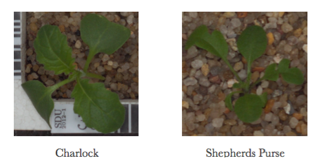
Can we distinguish a weed from a crop seedling? Many weeds and crop seedlings look similar, so sometimes it can be hard to differentiate the two. Although they look alike when they are young, they will eventually grow into totally different plants. This challenge presents itself in many real-world situations. For example, Charlock is an agricultural weed and an invasive species in some areas outside its native range, while Shepherds Purse, considered an herbal medicine, has seedlings of very similar shape to Charlock (See Fig1). Thus, farmers need to differentiate each type of seedling to successfully cultivate without damaging their plants. The goal of this project is to build a model to effectively classify several species of seedlings. This is based on a Kaggle project called “Plant Seedlings Classification” (https://www.kaggle.com/c/plant-seedlings-classification). The dataset contains 4,750 training images and 794 test images, each of which belongs to one of twelve species at several different growth stages. I aim to train several deep learning models using Python/Keras, and test how accurately they can estimate the correct species.
Problem Statement
Why is this project meaningful? As described earlier, many types of seedlings look very similar, so even an experienced gardener can have difficulty differentiating weeds from the seedlings of more helpful plants. Moreover, as each species includes different growth stages, the character of each seedling could change depending on their stage of growth. Furthermore, I will use low resolution images, which are more likely representative of real life, and because of their low resolution it is not always easy for even an experienced human to identify the correct seedling species.
This problem is related to a computer vision challenge, so I will leverage a Convolutional Neural Network (CNN) to train a model to categorize each seedling in the dataset. CNNs are particularly powerful for training on multi-dimensional data, such as images. They are designed to handle 2D spatial information in images particularly well; unlike a regular neural network, CNNs use locally-connected layers and do not use vectors for their hidden layers. To do this, I need to implement models with multiple trials with different CNN layers, such as convolution and pooling layers by using different optimizing parameters and dropout. Furthermore, I will compare my models from scratch with models using the popular technique of transfer learning with Xception, which has been established to help save time when training neural networks on image classification problems. Finally, I will determine the best model to predict seeding species using mean F-score as the evaluation metric, and I will elaborate on it in the following section.
Analysis
Data Exploration
The dataset contains 4,750 training images and 794 test images, each of which belongs to one of twelve species at several different growth stages. I obtained the dataset through a Kaggle competition, but originally the dataset was from the Aarhus University Department of Engineering Signal Processing Group. The training images include the label of seedling species, while the test images do not include labels. I am using only the 4,750 training images to train a model and validate and test the model accuracy.
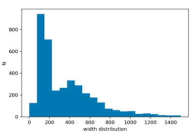
The input images are all square, but they have a wide range of pixel widths and heights, with some less than 100x100 pixels and some over 1000x1000 pixels, and each image has RGB colors. The figure on left (Fig2) shows the distribution of pixel widths (also equal to the height distribution) for all input images. I will need to rescale the input images to a uniform size to input into my neural network. A smaller uniform size makes the most sense, considering that many images are ~100 pixels on a side, and it’s easier to reduce the sizes of images than to reliably scale up the smaller images to a larger size. Also, using a smaller uniform size will help to save computational power. Therefore, I chose to rescale all images to the minimum size of the input data, 47 x 47.
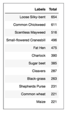
The input images include twelve seedling species from the following: Black-grass, Charlock, Cleavers, Common Chickweed, Common wheat, Fat Hen, Loose Silky-bent, Maize, Scentless Mayweed, Shepherds Purse, Small-flowered Cranesbill, Sugar beet. The table below gives the total number of each species, which range from 221 - 654.
I split the 4,750 images into three different datasets: training set ( 80%), validation set (10%), and a test set (10%). The training set is used to train the model and the validation set is used to adjust weight parameters to check the loss function after training the model. Finally, the test set serves to check the model accuracy using our scoring metrics. The images below are examples of each seedling of the input images.

As seen above (Fig3), the input images only include soil, gravel, and measure tape, except seedlings. So, filtering with other objects might not matter much. However, some seedlings, such as Black-grass, have pretty narrow leaves, so it might not be easy to train on those images. Also, some photos are blurry, so it could be hard to predict “by eye” as well. As mentioned earlier, as part of the pre-processing I rescale all input images to the minimum size of the input images, 47 x 47, which helps to save computational time.
Algorithms and Techniques
Why CNN? Neural Networks are designed to mimic the process of learning from the human brain. They can be comprised of multiple layers, each containing many nodes to simulate neurons. When training a neural network, the weights applied to each node are adjusted. A regular neural network connects every node to every other node in each successive layer, making them fully connected. To process an image with a regular neural network, the image must first be transformed into a vector. This transformation is not optimal for analyzing 2-D images because it uses a vector for each layer. On the other hand, CNNs are especially powerful when we must train on multi-dimensional data, such as images, because layers of a CNN have neurons arranged in 3 dimensions. CNNs consist of locally connected layers, which use far fewer weights compared to the densly connected layers of a regular neural network. The locally connected layers efficiently prevent overfitting and allow us to easily understand the image data because they naturally handle two dimensional patterns. You can read more details in the "Step 2-2. Define the CNN model architecture" in the previous blog, dog breed classifications.I will use a CNN to train a model using Keras in Python to categorize each seedling in the dataset. Keras is a deep learning library in Python, allowing for easy and fast prototyping. Keras allows one to build a model with a linear stack of layers, so I can quickly build a basic CNN structure with multiple layers and see how it performs. I will start with a basic CNN structure with three convolutional layers and pooling layers. Also, it will have a fully-connected layer with a softmax activation function before the output layer. Once the basic CNN is set up, I will improve the model in several ways such as:
- 1) adding more CNN layers
- 2) differentsizeoffilters
- 3) different optimization functions (SGD, Adam)
- 4) image augmentation
Finally, I will compare the results of the CNN models with the results I obtain using transfer learning, by building CNNs on top of the popular models, Xception.
Benchmark
For a benchmark model, I will use the simple CNN model described above with three convolutional layers and max-pooling layers. I tested this simple CNN on the input dataset, and I achieved a mean F-score of 0.40, and a prediction accuracy of 0.4. This accuracy is much better than random chance (1/12), but still not impressive. The aim of this project is to find a model with significantly better mean F-score and accuracy.
Methodology
Data Preprocessing
The data preprocessing function includes three processes as follows: First, the images are reshaped to have the same width and hight (47 pixels by 47 pixels). Second, I convert the image data to Numpy arrays with (number of images, 3, 47, 47). Also, I convert the pixel values to float32 format and normalize all of the arrays. In the case of the label dataset, I simply convert 1-dimensional class arrays to 12-dimensional class matrices. All codes for these are available in my github.
Implementation
Next, I start with a basic CNN structure with three convolutional layers and Max Pooling layers. Also, it will have fully connected layer with activation function (Relu) before the output layer. Finally, I added Global Average Pooling layers and a fully connected layer to predict the probabilities for each species. The code for this basic CNN structure is below:
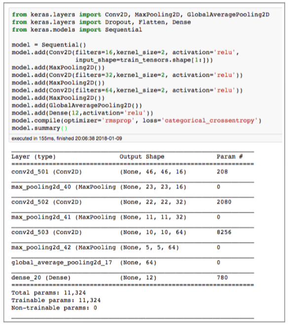
A callback is a set of functions to be applied at given stages of the training procedure. The code for my callback function implementation is below. For fitting a model, I used 10 epochs and 20 for the batch size.
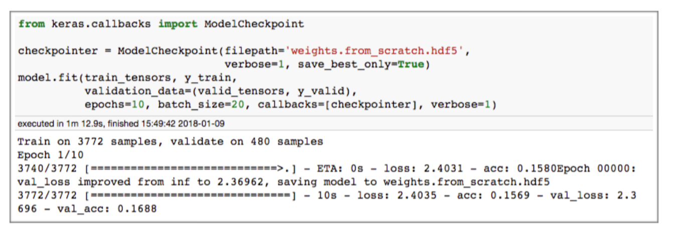
The mean F1 score of this first basic CNN is approximately 0.34, and accuracy is 0.4. I will use this as my benchmark model.
Refinement
Once the basic CNN is set up, I improved upon the model in several ways such as: (1) adding more CNN layers, (2) different size of filters, (3) different optimization functions (SGD, Adam), and (4) Image augmentation.
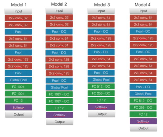
(1) I designed four different models shown in Fig8. One of the biggest challenges I faced was designing different models to test, because there are so many free parameters. I looked to other models people have used for inspiration in designing these four models in Fig8. For compiling these models, I used ‘categorical_crossentropy' as loss function and ‘Adam’ as optimizer with the default values of the parameters (e.g., learning rate=0.001). Then, I iterated each model with 20 epochs with batch_size=20 with training set and validation set. Another difficult challenge was determining a reasonable number of epochs to train these models, because I needed to find the right balance between saving time and getting reliable estimates for the performance of these models.
The following table gives the results of each model. The accuracy and mean F-1 score values are calculated with the test set, which I did not use to train models. The running time is estimated by my macbook, which has 2.9 GHz Intel Core i5.
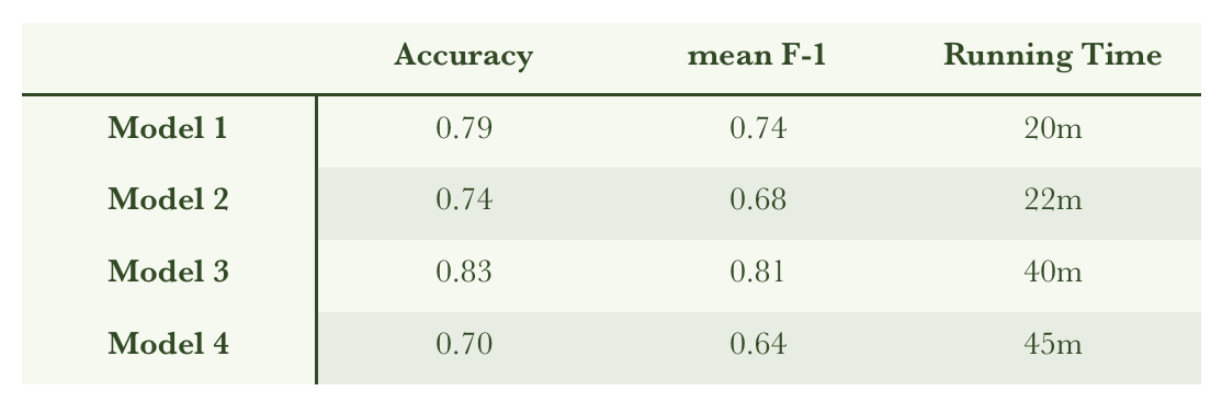
As seen above, Model 3 has the best result, with Accuracy=0.83 and mean F-1 score=0.81 with test data. However, when I compare the running time, Model 1 and Model 2 have much better time efficiency. Thus, I picked two models, Model 1 (best time efficiency with the second best mean F-1) and Model 3 (best mean F-1 value) to use in the next trial to refine my process.
(2) With Model 1 and Model 3, I trained them with a different filter size (3 x 3) compared to the original filter size (2 x 2). The table below compares the previous results to the new trials, with a larger filter size, for the two models I’m testing.
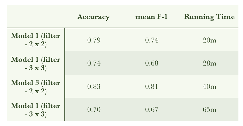
Overall, we can see there is no improvement for both models. So, I decided to use the first filter size (2 x 2) hereafter for my convolutional layers.
(3) I have used the Adam optimization algorithm with the default value for the learning rate. I decided to test my models using a range of learning rates: 0.01, 0.0005, and 0.0001. Also, I tried to use the Root Mean Square Propagation (RMSProps) as an alternative optimization algorithm. The results of these tests are in the table below.

Overall, the default value of the learning rate for Adam optimization function seems to be the best choice. The lower learning rates, like 0.0001, did not work well because it is too slow, and so it requires many more epochs to train the model. Considering the time efficiency, I concluded that a lower learning rate is not appropriate for the models. Also, I tried using a larger learning rate than 0.001 with the Adam algorithm, but most of them did not work well. So, I left those models off the table above. On the other hand, RMSProps works pretty well, but using Adam optimization function seems to have a slightly better result. Therefore, I decided to use an Adam optimization algorithm and used the Keras default values (e.g., lr=0.001).
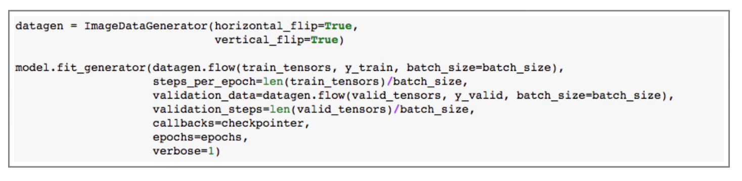
Finally, I added Image Augmentation, which is the process of taking images that are already in a training dataset and manipulating them to create many altered versions of the same images. For example, we can have more images with different rotation angles or vertically/horizontally flipped versions of the original images. This provides more images to train on, which could help a model to better generalize its training. The function ImageDataGenerator() in Keras generates batches of the input images with many different variations depending on its parameters. You can read more details here. .flow() and .fit_generator() are used to fit the model in batches with data augmentation. We can use these at the same time, as the code above shows. I only applied the horizontal_flip and vertical_flip options. This is my last refinement factor, so I trained the models with many epochs (30 - 50).
I took the best Model 1 in the table above, and the best Model 3 above, and then trained those models on an additional 30 epochs using image augmentation. The results of these tests are given in the table below.
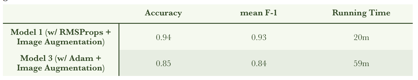
Model 1 results in a better accuracy and higher mean f1 score (even with less time). Therefore, I decided to use Model 1 with RMSProps + Image Augmentation. Having settled on a model, I next decided to train it using larger input image sizes ( 256 x 256) with 50 epochs. At the same time, for comparison I used a pre-trained Xception model with fully-connected layers added (to do transfer learning). As with the model above, I first trained the model with Xception without image augmentation, and then trained it with image augmentation. The table below has the results using Xception. It seems surprising that the Xception model performed slightly worse than the Model 1 results above, but this was mainly due to a limitation in my CPU power. The training of the Xception model, which took 200 min, only got through five epochs. If I had more time or a more powerful processor, I would have achieved better results through transfer learning. However, given my computational resources, I would choose to use Model 1 above to train a model for this project.
Result
The Model 1 (+RMSprops optimization and Image Augmentation) is my final chosen CNN model made from scratch. The code for the model is saved on my Github page (Here).
Model Evaluation and Validation
The table in the previous section has my final accuracy (0.94) and mean F-1 value (0.93) of the model using the test sets. The result is a vast improvement over the first CNN model that I tried, especially considering that the total run time is less than 30 min on my macbook. The inclusion of image augmentation in my final model allows that model to better generalize the training dataset, and therefore to achieve better accuracy in the test dataset.
Justification
- Benchmark model : mean F1 score is 0.34, and accuracy is 0.4
- Final model : mean F1 score is 0.93, and accuracy is 0.94
The comparison between my bench mark model and the final model shows that I have more than doubled my accuracy, and the F1 score is nearly triple.
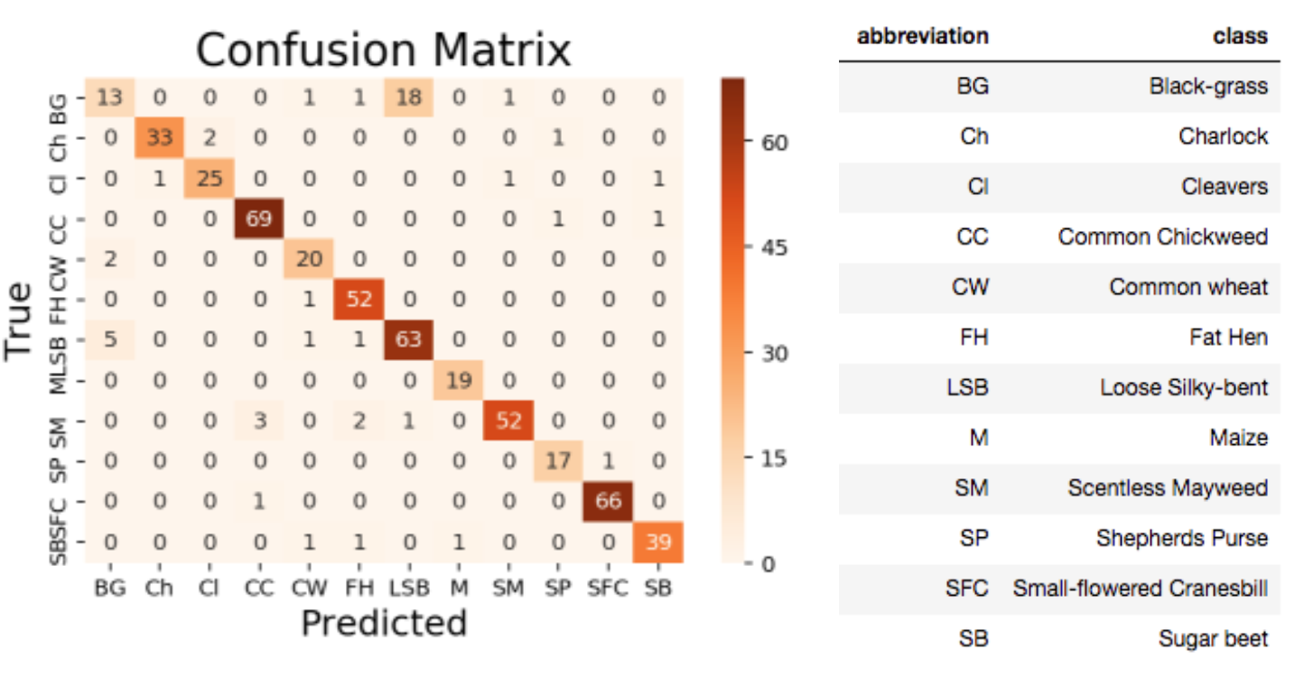
Above I plot the confusion matrix to more closely analyze the results of the model. The x-axis is the predicted class and y-axis is the true class for 10% seedings of overall sample (the test sample). The diagonal numbers correspond to the cases where the predicted class is matched with the true classes. The sum of each row gives the TNs (True Negatives), which are called “Negative” although the seedlings are truly identified. The sum of each column gives the FPs (False Positives), which although they are called “Positive”, the seedlings are falsely identified. Thus, Precision and Recall are each 0.93. Based on the definition of mean F-1 score I mentioned in the previous section, I derive 0.93 as mean F-1 score. The equations used to explicitly calculate these are given later in this section.
In order to check the result in detail, I compared TP, FP, TN, Precision, and Recall for each seeding species. The table below shows the results. As you can see, most of the seedling species are relatively well-recognized by the model, with the obvious exception being BG (which is often mis-identified as LSB).
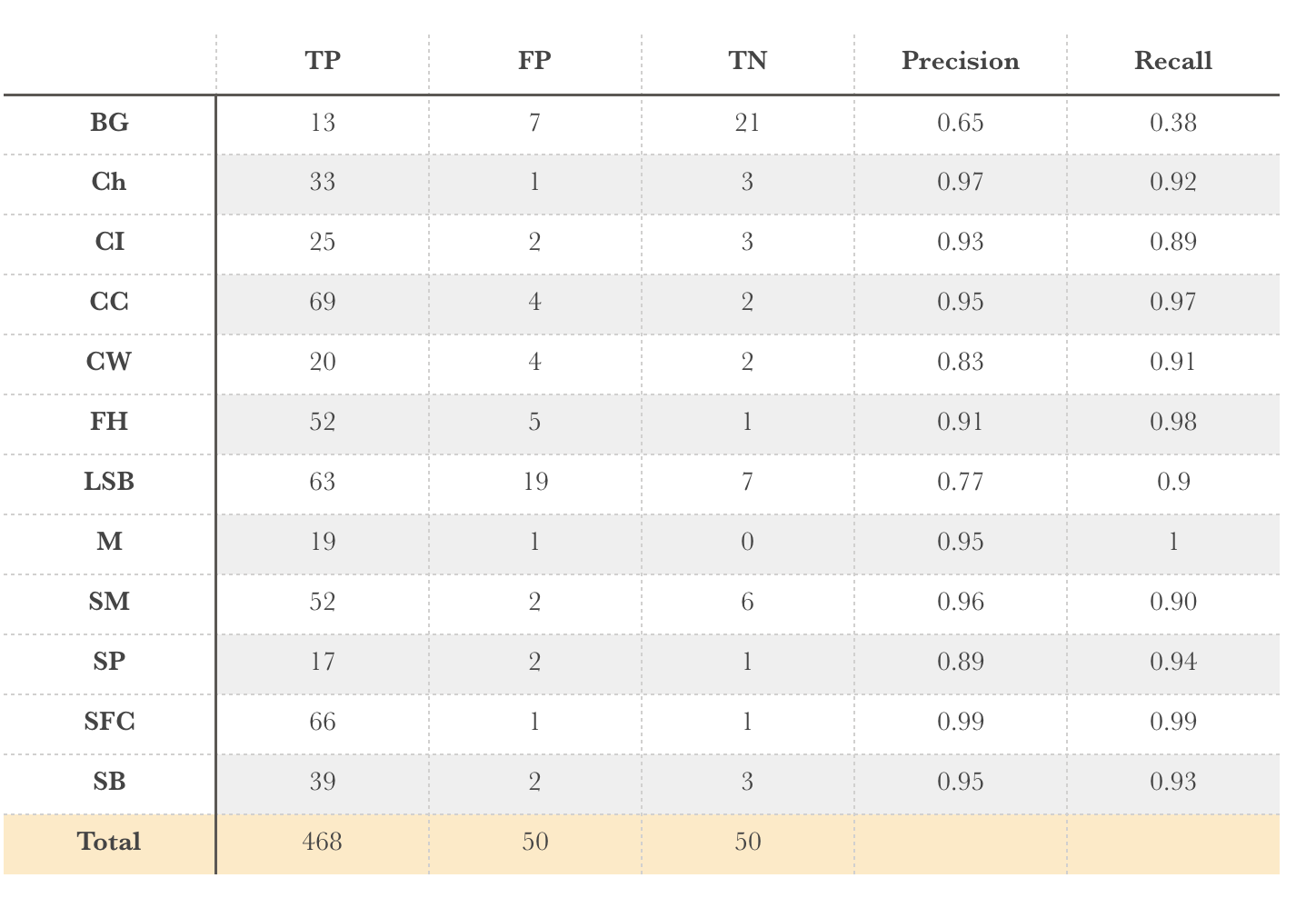
Here, I use the micro-average mean F-1 score, which is given by:
- Precision = (TP1+TP2+…+TP12) / (TP1+TP2+……+TP12 + FP1 + FP2 +…. +FP12)
- Recall = (TP1+TP2+…+TP12) / (TP1+TP2+…+TP12 + FN1 + FN2 +…. +FN12)
Thus, precision & recall are 0.93, and F-1 score is the same.
Summary and Future work
End-to-End Summary
I tested a variety of different CNN models, using different numbers of filters, sizes of filters, optimization functions, and with or without image augmentation. I also used a pre-trained model (based on Xception) as a comparison to my CNN built from scratch, and I found the results to be slightly better with the pre-trained model. Both of my refined models have significantly better results when compared to the first basic model with three simple convolutional layers. I verified the test score using the leaderboard on Kaggle, so I got the result of 0.93 using their test data.
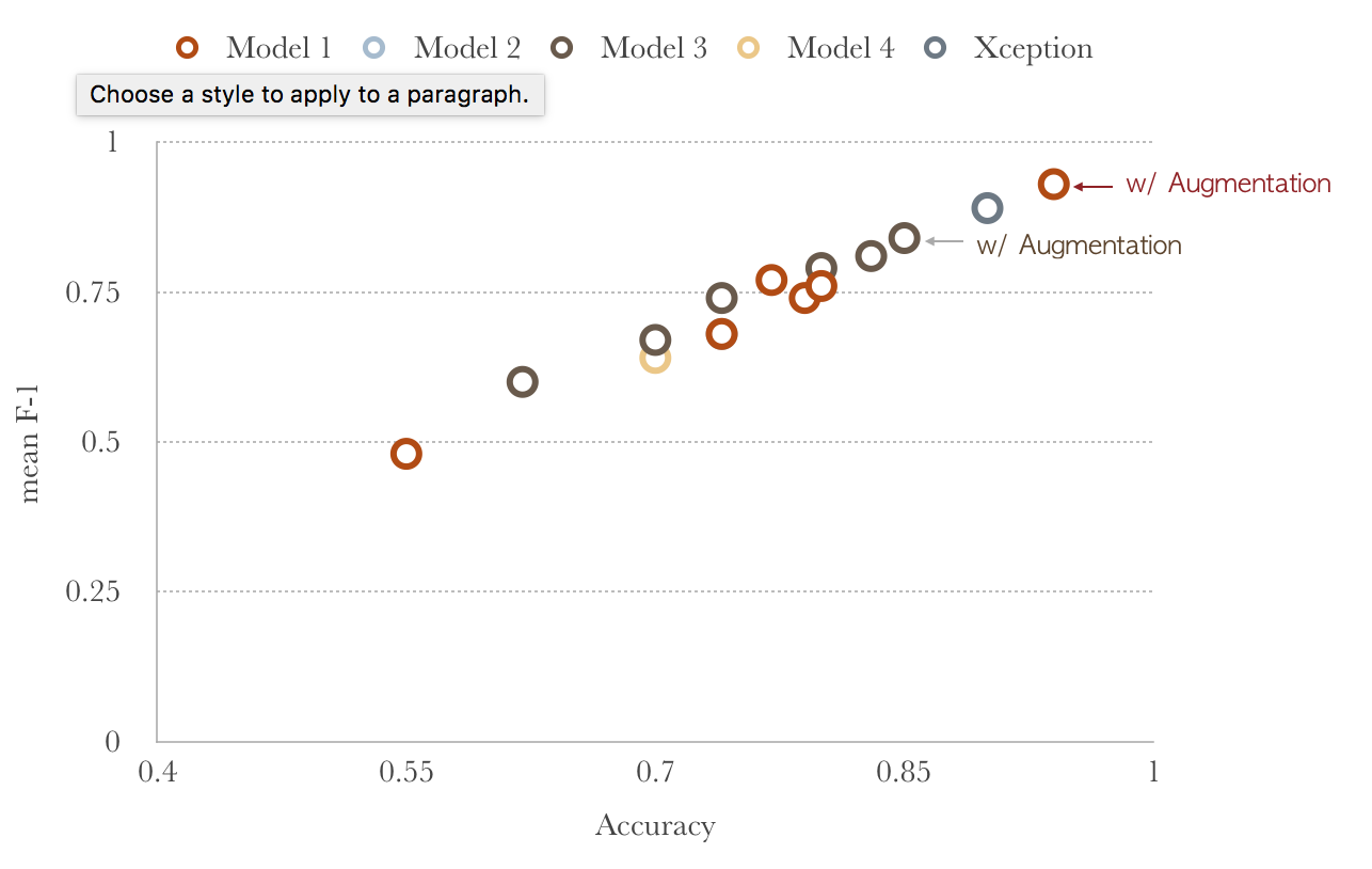
The figure above shows the F-1 score vs. accuracy for all of the models tested in this project. Different colored symbols indicate the different model tested. This figure highlights the significant improvements made with the variation in the models that were tested. Furthermore, the linear trend results from the fact that F-1 score correlates with accuracy.
Reflection
One of the biggest challenges for me in the project was the sheer number of free parameters available when building a CNN from scratch. It was hard for me to even know where to start in testing a set of models, and the fact that training each one takes at least 20 minutes only added to the difficulty. However, I came away from this process with a much greater understanding of what each of these components of a CNN does, and the effects they have on the computational time and on the final qualities of the models. So my take-away from this project will certainly be that the process of testing out all of these models was really valuable for me. I also have a greater appreciation of the value of using Cloud Computing (e.g., AWS) with GPU processors, which would allow me to more rapidly prototype model variations to speed up this process in the future.
Improvement
(1) When examining the confusion matrix above, the most obvious flaw is the mis-identification between Black-grass (BG) and Loose silky-bent (LSB). The precision and recall for Black-grass is the worst overall, since a large fraction of the BG are considered by the model to be LSB. On the other hand, the precision and recall for LSB are not bad, because I believe the number of input images for LSB could be enough to train the model to predict with at least a 90% accuracy. Thus, the most important step I would take to improve my model would be to include more images, especially for the BG class. At the same time, if we want to use this model to categorize BG, we need to accept that there will be a significant number of FPs and TNs (and a lower precision and recall). If you look back at Fig3, which shows example images of each seedling species, it’s apparent that the features of BG are not very easy to see, and that visually they look very similar to the LSB seedlings. This no doubt contributes to the problems that the model has with identifying them.
Cloud : Everything in this project was executed on my laptop, which is not the most efficient way to train models such as these. In the future, I will use GPU computing on an Amazon Web Services EC2 instance, which can be extremely helpful because it will allow me to train more models, and with a greater number of epochs, thanks to a large improvement in speed. On AWS, I could also use larger image input sizes than 47x47. Also, I could test many pre-trained models with different parameters, which could also lead me find a better overall model.
Reference
- https://www.kaggle.com/c/plant-seedlings-classification
- https://www.tensorflow.org/tutorials/layers
- https://machinelearningmastery.com/adam-optimization-algorithm-for-deep-learning/
- https://towardsdatascience.com/image-augmentation-for-deep-learning-using-keras-and-histogram-equalization-9329f6ae5085
- https://www.kaggle.com/gaborfodor/seedlings-pretrained-keras-models
- https://keras.io/applications/
- http://cs231n.github.io/convolutional-networks/#overview